 Measuring the size of an object (or objects) in an image has been a heavily requested tutorial on the PyImageSearch blog for some time now — and it feels great to get this post online and share it with you.
Today’s post is the second in a three part series on measuring the size of objects in an imageand computing the distances between them.
Last week, we learned an important technique: how reliably order a set of rotated bounding box coordinates in a top-left, top-right, bottom-right, and bottom-left arrangement.
Today we are going to utilize this technique to aid us in computing the size of objects in an image. Be sure to read the entire post to see how it’s done!
Looking for the source code to this post?
Jump right to the downloads section.
Measuring the size of objects in an image with OpenCV
Measuring the size of objects in an image is similar to computing the distance from our camera to an object — in both cases, we need to define a ratio that measures the number of pixels per a given metric.
I call this the “pixels per metric” ratio, which I have more formally defined in the following section.
The “pixels per metric” ratio
In order to determine the size of an object in an image, we first need to perform a “calibration” (not to be confused with intrinsic/extrinsic calibration) using a reference object. Our reference object should have two important properties:
- Property #1: We should know the dimensions of this object (in terms of width or height) in a measurable unit (such as millimeters, inches, etc.).
- Property #2: We should be able to easily find this reference object in an image, either based on the placement of the object (such as the reference object always being placed in the top-left corner of an image) or via appearances (like being a distinctive color or shape, unique and different from all other objects in the image). In either case, our reference should should be uniquely identifiable in some manner.
In this example, we’ll be using the United States quarter as our reference object and throughout all examples, ensure it is always the left-most object in our image:
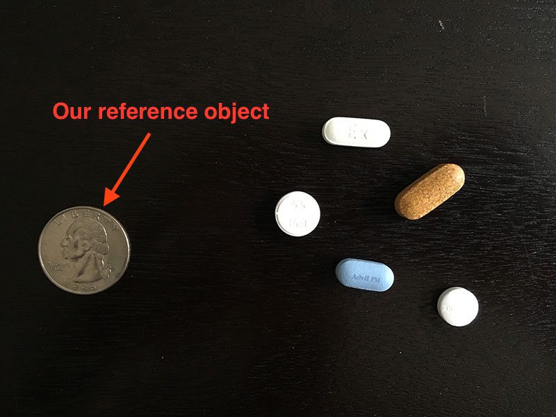
Figure 1: We’ll use a United States quarter as our reference object and ensure it is always placed as the left-most object in the image, making it easy for us to extract it by sorting contours based on their location.
By guaranteeing the quarter is the left-most object, we can sort our object contours from left-to-right, grab the quarter (which will always be the first contour in the sorted list), and use it to define our pixels_per_metric, which we define as:
pixels_per_metric = object_width / know_width
A US quarter has a known_width of 0.955 inches. Now, suppose that our object_width(measured in pixels) is computed be 150 pixels wide (based on its associated bounding box).
The pixels_per_metric is therefore:
pixels_per_metric = 150px / 0.955in = 157px
Thus implying there are approximately 157 pixels per every 0.955 inches in our image. Using this ratio, we can compute the size of objects in an image.
Measuring the size of objects with computer vision
Now that we understand the “pixels per metric” ratio, we can implement the Python driver script used to measure the size of objects in an image.
Open up a new file, name it object_size.py , and insert the following code:
Measuring size of objects in an image with OpenCV
Python
1
2
3
4
5
6
7
8
9
10
11
12
13
14
15
16
17
18
19 |
# import the necessary packages
from scipy.spatial import distance as dist
from imutils import perspective
from imutils import contours
import numpy as np
import argparse
import imutils
import cv2
def midpoint(ptA, ptB):
return ((ptA[0] + ptB[0]) * 0.5, (ptA[1] + ptB[1]) * 0.5)
# construct the argument parse and parse the arguments
ap = argparse.ArgumentParser()
ap.add_argument("-i", "--image", required=True,
help="path to the input image")
ap.add_argument("-w", "--width", type=float, required=True,
help="width of the left-most object in the image (in inches)")
args = vars(ap.parse_args()) |
Lines 2-8 import our required Python packages. We’ll be making heavy use of the imutils package in this example, so if you don’t have it installed, make sure you install it before proceeding:
Measuring size of objects in an image with OpenCV
Shell
Otherwise, if you do have imutils installed, ensure you have the latest version, which is0.3.6 at the time of this writing:
Measuring size of objects in an image with OpenCV
Shell
| 1 |
$ pip install --upgrade imutils |
Lines 10 and 11 defines a helper method called midpoint , which as the name suggests, is used to compute the midpoint between two sets of (x, y)-coordinates.
We then parse our command line arguments on Lines 14-19. We require two arguments, --image , which is the path to our input image containing the objects we want to measure, and--width , which is the width (in inches) of our reference object, presumed to be the left-most object in our --image .
We can now load our image and preprocess it:
Measuring size of objects in an image with OpenCV
Python
21
22
23
24
25
26
27
28
29
30
31
32
33
34
35
36
37
38
39
40 |
# load the image, convert it to grayscale, and blur it slightly
image = cv2.imread(args["image"])
gray = cv2.cvtColor(image, cv2.COLOR_BGR2GRAY)
gray = cv2.GaussianBlur(gray, (7, 7), 0)
# perform edge detection, then perform a dilation + erosion to
# close gaps in between object edges
edged = cv2.Canny(gray, 50, 100)
edged = cv2.dilate(edged, None, iterations=1)
edged = cv2.erode(edged, None, iterations=1)
# find contours in the edge map
cnts = cv2.findContours(edged.copy(), cv2.RETR_EXTERNAL,
cv2.CHAIN_APPROX_SIMPLE)
cnts = imutils.grab_contours(cnts)
# sort the contours from left-to-right and initialize the
# 'pixels per metric' calibration variable
(cnts, _) = contours.sort_contours(cnts)
pixelsPerMetric = None |
Lines 22-24 load our image from disk, convert it to grayscale, and then smooth it using a Gaussian filter. We then perform edge detection along with a dilation + erosion to close any gaps in between edges in the edge map (Lines 28-30).
Lines 33-35 find contours (i.e., the outlines) that correspond to the objects in our edge map.
These contours are then sorted from left-to-right (allowing us to extract our reference object) on Line 39. We also initialize our pixelsPerMetric value on Line 40.
The next step is to examine each of the contours:
Measuring size of objects in an image with OpenCV
Python
42
43
44
45
46
47
48
49
50
51
52
53
54
55
56
57
58
59
60
61
62
63 |
# loop over the contours individually
for c in cnts:
# if the contour is not sufficiently large, ignore it
if cv2.contourArea(c) < 100:
continue
# compute the rotated bounding box of the contour
orig = image.copy()
box = cv2.minAreaRect(c)
box = cv2.cv.BoxPoints(box) if imutils.is_cv2() else cv2.boxPoints(box)
box = np.array(box, dtype="int")
# order the points in the contour such that they appear
# in top-left, top-right, bottom-right, and bottom-left
# order, then draw the outline of the rotated bounding
# box
box = perspective.order_points(box)
cv2.drawContours(orig, [box.astype("int")], -1, (0, 255, 0), 2)
# loop over the original points and draw them
for (x, y) in box:
cv2.circle(orig, (int(x), int(y)), 5, (0, 0, 255), -1) |
On Line 43 we start looping over each of the individual contours. If the contour is not sufficiently large, we discard the region, presuming it to be noise left over from the edge detection process (Lines 45 and 46).
Provided that the contour region is large enough, we compute the rotated bounding box of the image on Lines 50-52, taking special care to use the cv2.cv.BoxPoints function for OpenCV 2.4 and the cv2.boxPoints method for OpenCV 3.
We then arrange our rotated bounding box coordinates in top-left, top-right, bottom-right, and bottom-left order, as discussed in last week’s blog post (Line 58).
Lastly, Lines 59-63 draw the outline of the object in green, followed by drawing the vertices of the bounding box rectangle in as small, red circles.
Now that we have our bounding box ordered, we can compute a series of midpoints:
Measuring size of objects in an image with OpenCV
Python
65
66
67
68
69
70
71
72
73
74
75
76
77
78
79
80
81
82
83
84
85
86
87 |
# unpack the ordered bounding box, then compute the midpoint
# between the top-left and top-right coordinates, followed by
# the midpoint between bottom-left and bottom-right coordinates
(tl, tr, br, bl) = box
(tltrX, tltrY) = midpoint(tl, tr)
(blbrX, blbrY) = midpoint(bl, br)
# compute the midpoint between the top-left and top-right points,
# followed by the midpoint between the top-righ and bottom-right
(tlblX, tlblY) = midpoint(tl, bl)
(trbrX, trbrY) = midpoint(tr, br)
# draw the midpoints on the image
cv2.circle(orig, (int(tltrX), int(tltrY)), 5, (255, 0, 0), -1)
cv2.circle(orig, (int(blbrX), int(blbrY)), 5, (255, 0, 0), -1)
cv2.circle(orig, (int(tlblX), int(tlblY)), 5, (255, 0, 0), -1)
cv2.circle(orig, (int(trbrX), int(trbrY)), 5, (255, 0, 0), -1)
# draw lines between the midpoints
cv2.line(orig, (int(tltrX), int(tltrY)), (int(blbrX), int(blbrY)),
(255, 0, 255), 2)
cv2.line(orig, (int(tlblX), int(tlblY)), (int(trbrX), int(trbrY)),
(255, 0, 255), 2) |
Lines 68-70 unpacks our ordered bounding box, then computes the midpoint between the top-left and top-right points, followed by the midpoint between the bottom-right points.
We’ll also compute the midpoints between the top-left + bottom-left and top-right + bottom-right, respectively (Lines 74 and 75).
Lines 78-81 draw the blue midpoints on our image , followed by connecting the midpoints with purple lines.
Next, we need to initialize our pixelsPerMetric variable by investigating our reference object:
Measuring size of objects in an image with OpenCV
Python
89
90
91
92
93
94
95
96
97 |
# compute the Euclidean distance between the midpoints
dA = dist.euclidean((tltrX, tltrY), (blbrX, blbrY))
dB = dist.euclidean((tlblX, tlblY), (trbrX, trbrY))
# if the pixels per metric has not been initialized, then
# compute it as the ratio of pixels to supplied metric
# (in this case, inches)
if pixelsPerMetric is None:
pixelsPerMetric = dB / args["width"] |
First, we compute the Euclidean distance between the our sets of midpoints (Lines 90 and 91). The dA variable will contain the height distance (in pixels) while dB will hold our widthdistance.
We then make a check on Line 96 to see if our pixelsPerMetric variable has been initialized, and if it hasn’t, we divide dB by our supplied --width , thus giving us our (approximate) pixels per inch.
Now that our pixelsPerMetric variable has been defined, we can measure the size of objects in an image:
Measuring size of objects in an image with OpenCV
Python
99
100
101
102
103
104
105
106
107
108
109
110
111
112
113 |
# compute the size of the object
dimA = dA / pixelsPerMetric
dimB = dB / pixelsPerMetric
# draw the object sizes on the image
cv2.putText(orig, "{:.1f}in".format(dimA),
(int(tltrX - 15), int(tltrY - 10)), cv2.FONT_HERSHEY_SIMPLEX,
0.65, (255, 255, 255), 2)
cv2.putText(orig, "{:.1f}in".format(dimB),
(int(trbrX + 10), int(trbrY)), cv2.FONT_HERSHEY_SIMPLEX,
0.65, (255, 255, 255), 2)
# show the output image
cv2.imshow("Image", orig)
cv2.waitKey(0) |
Lines 100 and 101 compute the dimensions of the object (in inches) by dividing the respective Euclidean distances by the pixelsPerMetric value (see the “Pixels Per Metric”section above for more information on why this ratio works).
Lines 104-109 draw the dimensions of the object on our image , while Lines 112 and 113display the output results.
Object size measuring results
To test our object_size.py script, just issue the following command:
Measuring size of objects in an image with OpenCV
Shell
| 1 |
$ python object_size.py --image images/example_01.png --width 0.955 |
Your output should look something like the following:
Figure 2: Measuring the size of objects in an image using OpenCV, Python, and computer vision + image processing techniques.
As you can see, we have successfully computed the size of each object in an our image — our business card is correctly reported as 3.5in x 2in. Similarly, our nickel is accurately described as 0.8in x 0.8in.
However, not all our results are perfect.
The Game Boy cartridges are reported as having slightly different dimensions (even though they are the same size). The height of both quarters are also off by 0.1in.
So why is this? How come the object measurements are not 100% accurate?
The reason is two-fold:
- First, I hastily took this photo with my iPhone. The angle is most certainly not a perfect 90-degree angle “looking down” (like a birds-eye-view) at the objects. Without a perfect 90-degree view (or as close to it as possible), the dimensions of the objects can appear distorted.
- Second, I did not calibrate my iPhone using the intrinsic and extrinsic parameters of the camera. Without determining these parameters, photos can be prone to radial and tangential lens distortion. Performing an extra calibration step to find these parameters can “un-distort” our image and lead to a better object size approximation (but I’ll leave the discussion of distortion correction as a topic of a future blog post).
In the meantime, strive to obtain as close to a 90-degree viewing angle as possible when taking photos of your objects — this will help increase the accuracy of your object size estimation.
That said, let’s look at a second example of measuring object size, this time measuring the dimensions of pills:
Measuring size of objects in an image with OpenCV
Shell
| 1 |
$ python object_size.py --image images/example_02.png --width 0.955 |
Figure 3: Measuring the size of pills in an image with OpenCV.
Nearly 50% of all 20,000+ prescription pills in the United States are round and/or white, thus if we can filter pills based on their measurements, we stand a better chance at accurately identification the medication.
Finally, we have a final example, this time using a 3.5in x 2in business card to measure the size of two vinyl EPs and an envelope:
Measuring size of objects in an image with OpenCV
Shell
| 1 |
$ python object_size.py --image images/example_03.png --width 3.5 |
Figure 4: A final example of measuring the size of objects in an image with Python + OpenCV.
Again, the results aren’t quite perfect, but this is due to (1) the viewing angle and (2) lens distortion, as mentioned above.
Summary
In this blog post, we learned how to measure the size of objects in an image using Python and OpenCV.
Just like in our tutorial on measuring the distance from a camera to an object, we need to determine our “pixels per metric” ratio, which describes the number of pixels that can “fit” into a given number of inches, millimeters, meters, etc.
To compute this ratio, we need a reference object with two important properties:
- Property #1: The reference object should have known dimensions (such as width or height) in terms of a measurable unit (inches, millimeters, etc.).
- Property #2: The reference object should be easy to find, either in terms of location of the object or in its appearance.
Provided that both of these properties can be met, you can utilize your reference object to calibrate your pixels_per_metric variable, and from there, compute the size of other objects in an image.
In our next blog post, we’ll take this example a step further and learn how to compute the distance between objects in an image.
Be sure to signup for the PyImageSearch Newsletter using the form below to be notified when the next blog post goes live — you won’t want to miss it!