自学教程：Using the bottleneck features of a pre-trained network: 90% accuracy in a minute

Using the bottleneck features of a pre-trained network: 90% accuracy in a minute

A more refined approach would be to leverage a network pre-trained on a large dataset. Such a network would have already learned features that are useful for most computer vision problems, and leveraging such features would allow us to reach a better accuracy than any method that would only rely on the available data.

We will use the VGG16 architecture, pre-trained on the ImageNet dataset --a model previously featured on this blog. Because the ImageNet dataset contains several "cat" classes (persian cat, siamese cat...) and many "dog" classes among its total of 1000 classes, this model will already have learned features that are relevant to our classification problem. In fact, it is possible that merely recording the softmax predictions of the model over our data rather than the bottleneck features would be enough to solve our dogs vs. cats classification problem extremely well. However, the method we present here is more likely to generalize well to a broader range of problems, including problems featuring classes absent from ImageNet.

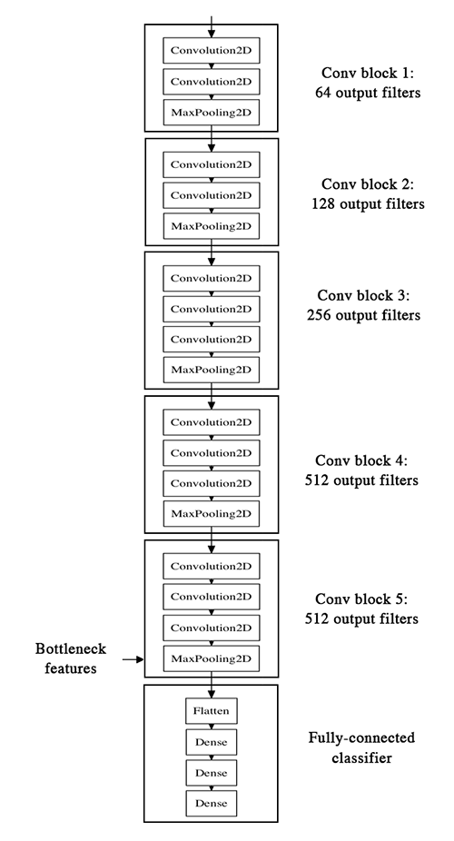
Here's what the VGG16 architecture looks like:

Our strategy will be as follow: we will only instantiate the convolutional part of the model, everything up to the fully-connected layers. We will then run this model on our training and validation data once, recording the output (the "bottleneck features" from th VGG16 model: the last activation maps before the fully-connected layers) in two numpy arrays. Then we will train a small fully-connected model on top of the stored features.

The reason why we are storing the features offline rather than adding our fully-connected model directly on top of a frozen convolutional base and running the whole thing, is computational effiency. Running VGG16 is expensive, especially if you're working on CPU, and we want to only do it once. Note that this prevents us from using data augmentation.

You can find the full code for this experiment here. You can get the weights file from Github. We won't review how the model is built and loaded --this is covered in multiple Keras examples already. But let's take a look at how we record the bottleneck features using image data generators:

batch_size = 16

generator = datagen.flow_from_directory(
        'data/train',
        target_size=(150, 150),
        batch_size=batch_size,
        class_mode=None,  # this means our generator will only yield batches of data, no labels
        shuffle=False)  # our data will be in order, so all first 1000 images will be cats, then 1000 dogs
# the predict_generator method returns the output of a model, given
# a generator that yields batches of numpy data
bottleneck_features_train = model.predict_generator(generator, 2000)
# save the output as a Numpy array
np.save(open('bottleneck_features_train.npy', 'w'), bottleneck_features_train)

generator = datagen.flow_from_directory(
        'data/validation',
        target_size=(150, 150),
        batch_size=batch_size,
        class_mode=None,
        shuffle=False)
bottleneck_features_validation = model.predict_generator(generator, 800)
np.save(open('bottleneck_features_validation.npy', 'w'), bottleneck_features_validation)

We can then load our saved data and train a small fully-connected model:

train_data = np.load(open('bottleneck_features_train.npy'))
# the features were saved in order, so recreating the labels is easy
train_labels = np.array([0] * 1000 + [1] * 1000)

validation_data = np.load(open('bottleneck_features_validation.npy'))
validation_labels = np.array([0] * 400 + [1] * 400)

model = Sequential()
model.add(Flatten(input_shape=train_data.shape[1:]))
model.add(Dense(256, activation='relu'))
model.add(Dropout(0.5))
model.add(Dense(1, activation='sigmoid'))

model.compile(optimizer='rmsprop',
              loss='binary_crossentropy',
              metrics=['accuracy'])

model.fit(train_data, train_labels,
          epochs=50,
          batch_size=batch_size,
          validation_data=(validation_data, validation_labels))
model.save_weights('bottleneck_fc_model.h5')

Thanks to its small size, this model trains very quickly even on CPU (1s per epoch):

Train on 2000 samples, validate on 800 samples
Epoch 1/50
2000/2000 [==============================] - 1s - loss: 0.8932 - acc: 0.7345 - val_loss: 0.2664 - val_acc: 0.8862
Epoch 2/50
2000/2000 [==============================] - 1s - loss: 0.3556 - acc: 0.8460 - val_loss: 0.4704 - val_acc: 0.7725
...
Epoch 47/50
2000/2000 [==============================] - 1s - loss: 0.0063 - acc: 0.9990 - val_loss: 0.8230 - val_acc: 0.9125
Epoch 48/50
2000/2000 [==============================] - 1s - loss: 0.0144 - acc: 0.9960 - val_loss: 0.8204 - val_acc: 0.9075
Epoch 49/50
2000/2000 [==============================] - 1s - loss: 0.0102 - acc: 0.9960 - val_loss: 0.8334 - val_acc: 0.9038
Epoch 50/50
2000/2000 [==============================] - 1s - loss: 0.0040 - acc: 0.9985 - val_loss: 0.8556 - val_acc: 0.9075

We reach a validation accuracy of 0.90-0.91: not bad at all. This is definitely partly due to the fact that the base model was trained on a dataset that already featured dogs and cats (among hundreds of other classes).

Fine-tuning the top layers of a a pre-trained network

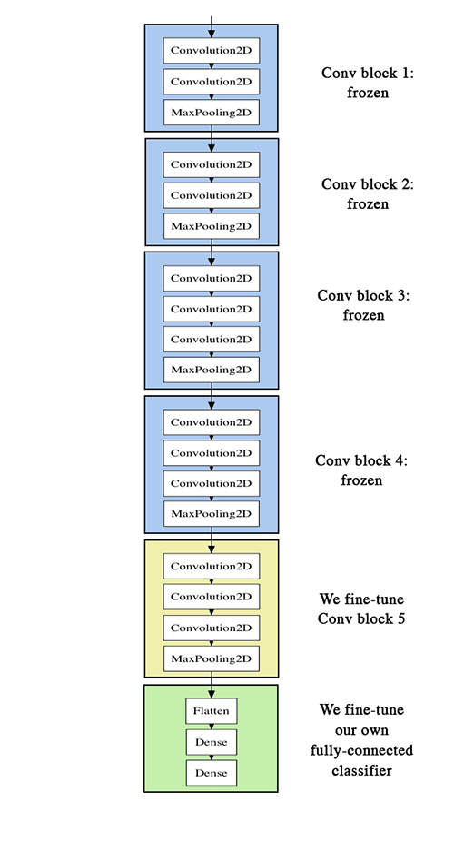
To further improve our previous result, we can try to "fine-tune" the last convolutional block of the VGG16 model alongside the top-level classifier. Fine-tuning consist in starting from a trained network, then re-training it on a new dataset using very small weight updates. In our case, this can be done in 3 steps:

• instantiate the convolutional base of VGG16 and load its weights
• add our previously defined fully-connected model on top, and load its weights
• freeze the layers of the VGG16 model up to the last convolutional block

Note that:

• in order to perform fine-tuning, all layers should start with properly trained weights: for instance you should not slap a randomly initialized fully-connected network on top of a pre-trained convolutional base. This is because the large gradient updates triggered by the randomly initialized weights would wreck the learned weights in the convolutional base. In our case this is why we first train the top-level classifier, and only then start fine-tuning convolutional weights alongside it.
• we choose to only fine-tune the last convolutional block rather than the entire network in order to prevent overfitting, since the entire network would have a very large entropic capacity and thus a strong tendency to overfit. The features learned by low-level convolutional blocks are more general, less abstract than those found higher-up, so it is sensible to keep the first few blocks fixed (more general features) and only fine-tune the last one (more specialized features).
• fine-tuning should be done with a very slow learning rate, and typically with the SGD optimizer rather than an adaptative learning rate optimizer such as RMSProp. This is to make sure that the magnitude of the updates stays very small, so as not to wreck the previously learned features.

You can find the full code for this experiment here.

After instantiating the VGG base and loading its weights, we add our previously trained fully-connected classifier on top:

# build a classifier model to put on top of the convolutional model
top_model = Sequential()
top_model.add(Flatten(input_shape=model.output_shape[1:]))
top_model.add(Dense(256, activation='relu'))
top_model.add(Dropout(0.5))
top_model.add(Dense(1, activation='sigmoid'))

# note that it is necessary to start with a fully-trained
# classifier, including the top classifier,
# in order to successfully do fine-tuning
top_model.load_weights(top_model_weights_path)

# add the model on top of the convolutional base
model.add(top_model)

We then proceed to freeze all convolutional layers up to the last convolutional block:

# set the first 25 layers (up to the last conv block)
# to non-trainable (weights will not be updated)
for layer in model.layers[:25]:
    layer.trainable = False

# compile the model with a SGD/momentum optimizer
# and a very slow learning rate.
model.compile(loss='binary_crossentropy',
              optimizer=optimizers.SGD(lr=1e-4, momentum=0.9),
              metrics=['accuracy'])

Finally, we start training the whole thing, with a very slow learning rate:

batch_size = 16

# prepare data augmentation configuration
train_datagen = ImageDataGenerator(
        rescale=1./255,
        shear_range=0.2,
        zoom_range=0.2,
        horizontal_flip=True)

test_datagen = ImageDataGenerator(rescale=1./255)

train_generator = train_datagen.flow_from_directory(
        train_data_dir,
        target_size=(img_height, img_width),
        batch_size=batch_size,
        class_mode='binary')

validation_generator = test_datagen.flow_from_directory(
        validation_data_dir,
        target_size=(img_height, img_width),
        batch_size=batch_size,
        class_mode='binary')

# fine-tune the model
model.fit_generator(
        train_generator,
        steps_per_epoch=nb_train_samples // batch_size,
        epochs=epochs,
        validation_data=validation_generator,
        validation_steps=nb_validation_samples // batch_size)

This approach gets us to a validation accuracy of 0.94 after 50 epochs. Great success!

Here are a few more approaches you can try to get to above 0.95:

• more aggresive data augmentation
• more aggressive dropout
• use of L1 and L2 regularization (also known as "weight decay")
• fine-tuning one more convolutional block (alongside greater regularization)

This post ends here! To recap, here is where you can find the code for our three experiments:

• Convnet trained from scratch
• Bottleneck features
• Fine-tuning